Machine Learning: Chapter 4 - Neural Networks
In this chapter we’re going to be diving into Neural Networks. Neural networks are a popular way to represent models that have many input variables. They’re a useful way to compose large complicated expressions that allow models to represent complex relationships between their inputs and outputs. To start off, though, let’s go back to our trusty productivity vs espressos model.
To briefly recap, on the left, we have our data points along with a drawing of the fit line. On the right, we have the loss vs slope chart along with the position indicated by the slider. In addition, we’re drawing the “gradient“ we discussed last time which indicates which way we should nudge the slider in order to improve the loss.
Let’s say we saw that other things impacted our productivity aside from how many espressos we drank. For example, whether or not we exercised in the morning, what we had for breakfast and how much sleep we had the night before all had an impact on productivity as well and we want to extend the model to include these values too.
Our initial formula was simple. We just multiplied the number of espressos by a factor, the slope and added a constant (the y intercept). Now let’s extend it to include the new parameters. We quickly run into a problem, though. How do we put “yes I exercised” or “I ate an omelette with red peppers” into a mathematical formula?
Representation of Variables
One challenge for machine learning tasks is deciding how to represent one of your input variables or predictors. In the case of the exercise, you could decide to represent it as a 1 or 0 value or potentially you might want to represent it as the number of minutes exercised. For the food, you could enumerate every possible breakfast meal as its own predictor. Then when translating that into the representation into the equation you would similarly do a one or zero value for each one of the foods depending on which you had eaten. Alternatively, you could consider distilling the foods that you’ve eaten into their nutrients (how many grams of fat, carbs and protein they consist of) and entering that into the model.
I’m going to level with you and tell you that I can’t say which of these approaches is the best but the main thing that I keep in mind as for whether it will be a good approach is something called the Bias-Complexity Tradeoff.
Briefly, the Bias-Complexity tradeoff states that the more complicated your model is, the better it will be able to learn complex relationships but the more data / longer it will take to learn. In addition, there is a risk that a more complex model will overfit to the data points given. Overfitting is a problem where the model makes mistaken assumptions based on the input data.
To express how this applies to representations of input variables let’s think of the approach of enumerating all possible input meals. This scheme has the possibility of doing a better job of learning things that are special to the meals that people are eating but it suffers from the problem that if the meals eaten are heterogeneous there may only be very few data points to learn anything about a meal from.
On the other hand, if you break down food into the amount of carbs, fat and protein, you’re giving yourself more data to work with but the problem is you’re introducing the implicit assumption (or bias) that all carbs, fat and protein are the same regardless of what form they come in which may or may not be a valid assumption.
Based on the variables I’m interested in I’m going to represent exercise as a one or a zero and represent the food I’ve eaten with the amount of fat, carbs and protein. So our full list of predictors is:
Number of espressos
Number of hours slept the night before
Whether or not I went to the gym in the morning
Breakfast nutrients (in grams):
Fat
Carbs
Protein
Let’s assume, for the sake of simplicity, that our estimate for productivity is a linear combination of all of those input variables.
Neural Networks
Our initial formula was:
\[y=mx + b\]
where x is the number of espressos drank. Typically the amount you multiply a predictor by is referred to as a bias, so instead of m we’ll use b and since there are more than one we’re going to denote them with a suffix.
\[ \hat{y} = w_0x_0 + b \]
So given that now we have 6 predictors the formula will be:
As you can see, writing equations this way can start to get unwieldy as the number of parameters grows.
As I mentioned at the beginning of the post, neural networks are a convenient way to compose complex relationships and they can easily be represented visually.
Let’s look at this formula represented as a neural network.
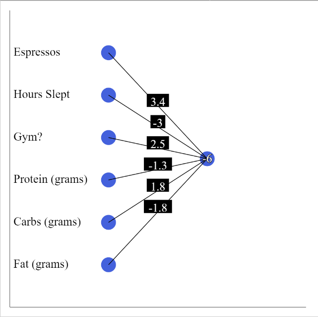
In this image, the neurons on the left represent the values for each of the predictors, number on the edges connecting the input neurons to the output neuron represent the weights and, finally, the output neuron includes the value b which is the y-intercept from the early examples.
The value of the output neuron is the same as the equation above. This is just another way to visualize it.
Now that we have a function of 6 variables, it won’t be possible for us to draw a real representation of the data but what we can do is visualize the loss since it’s still just a single number. And actually the loss function is pretty much unchanged aside from the fact that there are now 6 dimensions instead of 1. We calculate the output y given the input variables of each data point and compare that to the observed value and finally we square that value.
Expressed as a summation, the loss function looks like this:
where n is the number of data points that you have, y is the observed productivity for that data point and y-hat is the model’s prediction.
The last change to the demo is that we’re going to show the loss as a function of steps as opposed to a function of the input variables since, as mentioned before, it’s a high dimensional space which isn’t easy to visualize.
These are the knobs that a machine learning network is working with to optimize the loss given the particular input data.
Admittedly the default settings aren’t very interesting but try setting the sliders to extreme values and step using the gradient. Can you achieve a better loss than by starting with the default weights and bias of zero?
As you can see, this neural network is not too different from our initial example where we were we’re moving the sliders to try to fit the line, it’s just that there’s more sliders.
And as with the case in the gradient descent blog post, we can take the gradient to get a hint about which direction we should nudge all of these sliders.
To sum up the main takeaways:
Neural networks are a visual metaphor for large mathematical expressions
Training the neural network is just picking the values for all the sliders, there are just more of them
The caveat is that more sliders require more data.
Gradient descent works the same way as in fewer dimensions where it tells you which way you should nudge your sliders.
Up until this point I’ve been very hand-wavy about the gradient and how we find it but in the next post I’ll dive into a technique that’s called back propagation which is how the gradient is calculated for deeper neural networks.