ML: Chapter 2 - A closer look at loss with Linear Regression
Some of you may be thinking… Ugh linear regression? I thought this was supposed to be about Machine learning? Others of you may be thinking hmmm, that sounds familiar but I don’t recall the details. Some of you may have no idea what linear regression is. Well allow me to stop enumerating the hypothetical mental states of my readers and give a quick recap. Feel free to skip the next section if you’re already in the know. Regardless, I promise this will tie back to machine learning!
What is linear regression?
Let’s say you have some historical data about your perceived productivity on a particular day, given how many espressos you’ve had that day and you want a model you can use to predict productivity in the future.

Productivity is measured abstractly on a scale from 1 - 10, 10 being most productive.
Given this data, you could ask your spreadsheet software to calculate a “line of best fit”. This will create a simple line that tries to best approximate the data. That’s really all linear regression is. Let’s give that a shot:
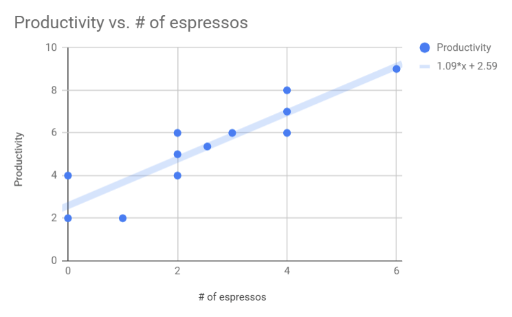
Okay so now we have a function we can use to estimate productivity given a particular number of espressos. In the key to the right we see that the equation for the fit line is 1.09x + 2.59. So, if you drank 5 espressos, the linear model here estimates that your productivity will be about 8/10. Useful information for deciding what you should order from the barista!
How did the software pick that equation? The rest of this blog post aims to build up an intuitive understanding of how the program is finding that line of best fit by using loss as the guiding principle and providing interactive examples that you can play around with.
Loss in the context of Linear Regression
The first thing I’d like to demonstrate are the two parameters that there are to tweak when performing a linear regression. Use the sliders below to adjust the y-intercept and slope of the fit line.
The main thing to keep in mind with the example above is that any fit line is defined by two parameters, the slope and the y-intercept. Since creating a linear model consists of just picking values for those parameters, it’s considered a parametric model.
You were probably able to pick pretty good values just by eyeing it up. Unfortunately, since the computer can’t “see” in the traditional sense, we need to give it some more help. So the next question is how do we pick these parameters without estimating by sight?
In math class, this would be the point at which a teacher would pull out a big ugly formula to calculate the slope and y-intercept and just say “Trust me, this is how you calculate it”.

I don’t know about you but these equations don’t mean much to me...
But our goal is to better understand how we can use loss to find these values instead of just calculating them.
Ultimately, we need a way to tell how good or bad a particular combination of slope and y-intercept is. This is where our loss function comes in. It’s responsible for taking a set of parameters and telling us how good they are. Even if we’re not 100% sure how to write a good loss function, one useful place to start is looking at how far the points are away from the value predicted by the fit line.
In the tool below, we’ve drawn the distance between the each point and our fit line. This distance is known as the residual.
Perhaps it goes without saying but we’d like these residuals to be as small as possible. Since we’re looking for a function that is higher when the model is worse, one thing to try is to add up all these residuals. This way, if a slope and y-intercept produce a line that is far from the points, the loss function will output correspondingly high values (indicating a bad model).
This is what we’ve done below. For each point, we’ve drawn the amount it contributes (or the penalty) to the value of the loss function. In addition, we’ve added the total penalty, over to the right. This box is the same area as all of the penalties of the points put together. It is a visual representation of the output of our loss function.
Awesome! Now we have something that the computer can work with. We have a single number that allows us to understand how well one particular combination of slope and y-intercept fits the data. By dragging the sliders around and looking at the size of the penalty, you are simulating an exploration of the space of parameters and evaluating the loss function at that point.
Before we get too excited, though, this loss function has a problem. Look at the example below. Try different values of the y-intercept. Keep on eye on the size of the total penalty when the fit line is between the upper and lower points. (Note: We’ve restricted the slope to illustrate the problem)
Did you notice that the total penalty didn’t change when the line was between the two sets of points? That’s an issue. Since the computer just has that one number to tell which is the best, it will have no way of choosing from any line of best fit that sits between the points.
So how can we make a loss function that incentivizes the computer to split the difference? Put another way, how can we add more to the total penalty for points that are particularly far away from the line of best fit?
One way to do that is to square the value of each residual before summing them together. The example below uses squared residuals as penalties as opposed to just the residuals. Do the same thing as above and keep on eye on the total penalty. At what point does the total penalty seem to be the smallest.
This new loss function should do a better job of “finding” the best line of fit. This is the loss function that is used, (indirectly) by Excel or Google Sheets when you create a line of best fit.
It’s important to point out, in regards to finding the minimal loss, we haven’t gotten all the way there. I’ve laid out the loss function and showed how the different values of the parameters map to values of the loss function. The missing part is the process of taking that loss function and finding the parameters that minimize it. That will have to be for a future blog post.
While typically most people wouldn’t think of performing a linear regression as ML, there are many useful parallels to draw:
We have a model
We can define a loss function to evaluate the model
We “train” the model to minimize the loss function
Other important takeaways are:
Not all loss functions are created equal, the best model as decided by a bad loss function might not be very good.
For parametric models, training amounts to selecting the values of the parameters to minimize loss.
[Reiteration] The loss function is a mapping from the values of the parameters to an abstract loss value, which represents how bad the model was, higher the loss, the worse the model.